Teaching an AI to invent new Chinese characters

For associated code, please see the github repo. Huge shoutout to my old friend Daniel Tse, linguist and ML expert extraordinaire for invaluable help and ideas on both fronts throughout this campaign.

In this article, we build a text-to-image AI that learns Chinese characters in the same way humans do - by understanding what their components mean. It can then invent new characters based on the meaning of an English prompt.

Intro

Chinese characters are pretty cool, and there are a lot of them; around 21,000 are represented in unicode alone. Interestingly, they encode meaning in multiple ways. Some are simple pictures of things - 山 (shān) means, as you might be able to guess, ‘mountain’. Most characters are compounds, however: 好 (hǎo), meaning ‘good’, is constructed from the pictograms for 女 (nǚ), ‘woman’ and 子 (zǐ), child. Read into that what you will. Compounds often contain a semantic and a phonetic component; these subcomponents are known as radicals. For example, the names of most metallic chemical elements such as lithium, 锂 (lǐ) are composed of a semantic radical (⻐, the condensed, simplified form of 金 (jīn) meaning ‘gold/metal’) and a phonetic component 里 (lǐ, of unrelated meaning) which approximates the ’li’ sound of lithium.

I’ve been interested for a while in how Chinese characters might be explored using machine learning. Can we teach a model to understand how they are structured from pictures and definitions alone? Can it then invent new characters? (Spoiler: yes) Let’s talk about a couple of ways of engaging with this, starting with relatively simple ML models and moving towards state-of-the-art technologies.

Dataset

First, we need a dataset consisting of images of as many known Chinese characters as possible. The unicode standard is a convenient method of indexing a large proportion of known Chinese characters. Fonts provide a specific way of representing characters, in the form of distinct glyphs. Fonts have different levels of completeness, so choosing one that contained as many characters as possible for a large and diverse dataset was important.

The main resources used for generating the dataset:

• The unicode CJK Unified Ideographs block (4E00–9FFF) of 20,992 Chinese characters
• Google fonts (Noto Sans and others)
• English definitions from the unihan database (kDefinition.txt) - this becomes useful later

Let’s make the dataset by saving the glyphs as pictures in the square 2ⁿ×2ⁿ format favoured by ML convention. We want to keep detail while minimizing size - I found that 64×64 and 128×128 worked well. Since we don’t need colour, we can get away with a single channel - otherwise we’d use a 3 channel RGB image of size 3×128×128.

Visualise the character set in 2D

(Jupyter notebook) First let’s map the space with a dimensional reduction. UMAP works well here. Distinct clusters emerge - the largest cluster on the left represents the “lefty-righty” characters (to use the technical term), while the second largest cluster on the right represents “uppy-downy” characters. Tighter clusters/subclusters tend to correspond to characters that share the same radical - the small streak at the very top right is an almost literal leper colony of characters with the 疒 radical, indicating sickness. (Hover over/tap points to see the characters)

Variational autoencoder

(Jupyter notebook) Let’s try using an older generative ML technology, the variational autoencoder (VAE), to model the underlying distribution of Chinese characters. The dimensionality of the original input boils down to a vector of length 64×64=4096, i.e. one value for each pixel. The VAE architecture works by using convolutional layers to reduce the dimensionality of the input over several steps (the ’encoder’), then using a reverse convolution to increase the dimensionality back to the original (the ‘decoder’). The network is trained on its ability to output a match to the original.

The key intuition is that not all of the pixels in the images contain valuable information, so they can somehow be compressed to a smaller (lower-dimensional) vector. This is known as the ’latent space’. By passing our training images through a bottleneck the size of the latent space and then training the model to reconstruct the full original image, we create a ‘decoder’ that can translate any vector in the latent space to a full sized image. In this case, we go from 64×64=4096 to a latent space of size 256.

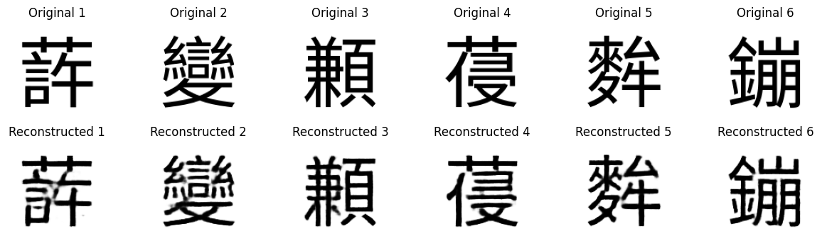
By passing images from our original dataset though the VAE again, we can see that the VAE has learnt a good latent representation of our glyphs:

Aside: Training the VAE has an extra subtlety compared to a vanilla autoencoder which is only graded on reconstruction. Our VAE loss function consists of not just reconstruction loss, but also the Kullback–Leibler divergence, which is a measure of distance between two probability distributions. In this case, we want to minimize the distance between the learned distribution of Chinese glyphs and the normal distribution N(0,I). This pushes the latent distribution from ‘whatever it wants to be’ towards a normal distribution, which makes sampling and traversing the latent space easier.

We can compare the latent space learnt by the VAE by passing the dataset through the VAE encoder only, generating a dataset of vectors in the latent space. We can then apply the same UMAP visualisation as before. While the lefty-righty and uppy-downy clusters from before still exist, you can see that the points have all been pushed closer to a (2D) normal distribution. Intuitively, adjacent points in this distribution are more likely to be similar - it’s ‘smoother’.

We can interact with the latent space via the encoder and decoder components of our trained VAE. For example, we can perform bilinear interpolation between 4 characters. We obtain the latent vector for each one by using the VAE encoder as before, then interpolate the intermediate vectors and decode them to images with VAE decoder.

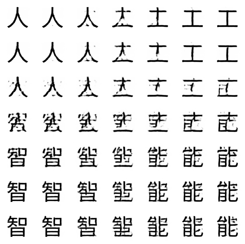
This allows us to do some interesting things like morph smoothly between characters by interpolating between vectors in latent space:

For some types of data such as faces or organic molecules, VAEs can be used to generate convincing new samples simply by moving around in the latent space. However, this is a dead end for us - the intermediate steps are clearly not valid Chinese characters, and there is no clear way of accessing the underlying structure of the distribution do so. This gives us a not-so-elegant segue to the generative modality du jour: diffusion models.

Unconditional diffusion model

Initially models designed to remove noise from images, it was found that when applied to pure noise, denoising diffusion models could generate entirely new images of types they were trained on. Even more excitingly, when trained with text conditioning, they could then generate images related to a provided text prompt. This led the proliferation of text-to-image models starting around late 2022 like Dall-E, Midjourney, Imagen, and Stable Diffusion. These models tend to be trained on a huge number of text-image pairs harvested en masse from the internet. The training cost of these models is generally on the order of 6 figures (USD) or more.

I was curious if the same type of architecture could be used in a simplified form, with a smaller dataset, to achieve an interesting result like generating convincing Chinese characters. Of course, I didn’t have 6 figures (USD) to spend on this - everything was done on my home rig with a used 3090 bought for ~$700 (the best VRAM Gb/$ value in 2023/4!).

The first step was to implement an unconditional model trained on our existing dataset, to see if convincing generations could be achieved at all. Unconditional simply means that the model is trained to generate similar things to the data it sees, without any other guidance. Those playing the home game can follow along with the associated notebook here

Most image diffusion models use some variant of the U-net architecture, initially developed for segmenting biomedical images. This network turns out to be a good choice for diffusion models, where we need to train a model that can predict noise that can then be subtracted to generate recognizable images. We also need a noise scheduler that controls the mathematics of how noise is added during the training process. To save time in implementing the whole model from scratch, we can use Huggingface’s handy diffusers library with the UNet2DModel for the Unet and the DDPMScheduler as the noise scheduler. This makes the core of the code relatively straightforward:

 1
 2
 3
 4
 5
 6
 7
 8
 9
10
11
12
13
14
15
16
17
18
19
20
21
22
23
24
25
26
27
28
29
30
31

from diffusers import UNet2DModel, DDPMScheduler

# Define the UNet model
model = UNet2DModel(
    sample_size=128,  # the target image resolution
    in_channels=1,  # the number of input channels
    out_channels=1,  # the number of output channels
    layers_per_block=2,  # how many ResNet layers to use per UNet block
    block_out_channels=(128, 128, 256, 256, 512, 512),  # the number of output channels for each UNet block

    # Define the UNet architecture
    down_block_types=(
        "DownBlock2D",
        "DownBlock2D",
        "DownBlock2D",
        "DownBlock2D",
        "AttnDownBlock2D",
        "DownBlock2D",
    ),
    up_block_types=(
        "UpBlock2D",
        "AttnUpBlock2D",
        "UpBlock2D",
        "UpBlock2D",
        "UpBlock2D",
        "UpBlock2D",
    ),
)

# Initialize the noise scheduler
noise_scheduler = DDPMScheduler(num_train_timesteps=1000)

As the process is relatively expensive, the large models mentioned above generally train on some kind of lower dimensional space, coupled with a method to later obtain high resolution images. For example, Google’s Imagen uses a sequence of conditioned superresolution networks, while Stable Diffusion is built on the idea of latent diffusion, where the final images are decoded from a lower-dimensional latent space using a VAE. This step is omitted here as we have enough compute to train the model in the relatively small native size (128×128) of the data. The remainder of the code is mostly plumbing to get the data to the model. I did run into a couple of traps here though:

1. The scheduler for running inference on a diffusion model need not be the same as the one used for training, and many good schedulers have been developed by the community that can give excellent results in 20-50 steps rather than the 100s that might be needed with the standard DDPMScheduler(). For our purposes, “DPM++ 2M” or DPMSolverMultistepScheduler() in the Diffusers library worked very well.

2. Dataloader shuffling is essential with such small datasets. I ran into a bug that took weeks to diagnose: sampling every epoch led to overfitting (lower training loss) with much poorer model performance as assessed by eye. The same model sampled every 10 epochs had no such problems. Test showed model parameters before and after sampling were identical. After much suffering, the problem was found to be caused by this inference call to the Diffusers pipeline I’d cribbed from Huggingface:

   1 2 3 4

   images = pipeline(batch_size=batch_size, generator=torch.manual_seed(config.seed), num_inference_steps=num_steps, ).images

   Setting generator=torch.manual_seed(config.seed) resets the seed for the whole training loop, meaning the model will see training samples in the same order every reset. This allowed the model to learn the sample order as an unintended side effect, leading to overfitting and degraded performance. Setting a generator on the CPU instead allows the training to continue unmolested: generator=torch.Generator(device='cpu').manual_seed(config.seed)

Below is a video of characters generated during each training epoch from a model trained for 100 epochs on the same Chinese glyph dataset used before. Compared to the VAE model discussed in the last part, we can see the unconditional diffusion model is much better at capturing the hierarchical structure of characters at different levels, and learns this very early on in the training process.

The model also works on other writing styles such as ancient Chinese seal script!

Conditional diffusion model

Now that we have confirmed a diffusion model can generate convincing Chinese characters, let’s train a text-to-image model conditioned on the English definitions of each character. If the model correctly learns how the English definition relates to the Chinese character, it should be able to ‘understand’ the rules for how characters are constructed and generate characters that ‘give the right vibe’ for a given english prompt.

In a previous blog post, I discussed finetuning Stable Diffusion. However that seemed like the wrong approach here - the pretraining of SD wouldn’t do much for us since the types of images we want to generate are unlikely to be well represented in their training set. So which framework to use?

In a misguided attempt to save effort, I first tried Assembly AI’s minimagen implementation, as an ostensibly simple conditional diffusion framework. It rapidly (but not rapidly enough) became clear that even after extensive debugging this was not fully functional demo code. I moved on to lucidrains’ much cleaner imagen implementation and trained some variants in unconditional mode, matching architectures as best as I could with my previous model (within the constraints of the framework), but I couldn’t never replicate the same quality - I suspect this was due to some differences in the layer architecture I couldn’t identify.

“You could not live with your own failure, where did that bring you? Back to me.”

In the end I decided I had to implement the model myself, something I’d been studiously avoiding. While huggingface’s UNet2DConditionModel() provides a framework for this, I was unable to find good documentation and so ended up having to scour the codebase directly. My observations below on what is needed, in case you dear reader want to take up this foolhardy task. Follow along with the notebook here.

The UNet2DConditionModel() is able to be conditioned on either discrete classes (dog, car, house, etc.), or embeddings (vectors from a latent space). For text-to-image, we are using embeddings. I decided to take a page out of Google’s book and use LLM embeddings directly for conditioning, as Imagen does. What Google found with Imagen was that conditioning on text embeddings from an LLM such as their T5 model worked just as well or even better than the CLIP model trained on image-caption pairs that Dall-E uses. This is very handy for us, since pretrained CLIP-type embeddings would likely be inappropriate for our use case reasons discussed above. In practice, we can call down existing T5 methods from Huggingface’s transformers library and pass it some text; it will give us back a fixed-length vector embedding, imbued with LLM magic.

Here’s the core of the conditional UNet model:

 1
 2
 3
 4
 5
 6
 7
 8
 9
10
11
12
13
14
15
16
17
18
19
20
21
22
23
24
25
26
27
28

from diffusers import UNet2DConditionModel

# Define the conditional UNet model
model = UNet2DConditionModel(
    sample_size=128,
    in_channels=1,
    out_channels=1,
    layers_per_block=2,
    block_out_channels=(128, 256, 512, 512),

    addition_embed_type="text", # Make it conditional
    cross_attention_dim=512,
    encoder_hid_dim=512,  # the hidden dimension of the encoder
    encoder_hid_dim_type="text_proj",
    
    down_block_types=(
        "DownBlock2D",
        "DownBlock2D",
        "CrossAttnDownBlock2D",
        "DownBlock2D"
    ),
    up_block_types=(
        "UpBlock2D",
        "CrossAttnUpBlock2D",
        "UpBlock2D",
        "UpBlock2D"
    ),
)

We specify the nature of the conditioning vector being passed to the model via some extra arguments. We also need to introduce some extra plumbing. First, we now need text captions for each training image, which we obtained from the unihan definitions database (way back at the top of this article). We then need a collator function that helps the dataloader return LLM embeddings from the text caption, as well as an attention mask for the embedding. Finally, we write our own pipeline, GlyffuserPipeline() (a subclass of DiffusionPipeline()) that can correctly pass the text embeddings and masks during inference. From there, we can train it in the same way as the previous model.

Learning the structure of Chinese characters

Now that we’ve trained the conditional model, how can we know what the model has learnt about how Chinese characters are constructed? One way is to probe it with different prompts and look at how the sampling steps progress. In the intro I mentioned that most characters contain semantic or phonetic radicals, and the UMAP shows the distribution of major character types.

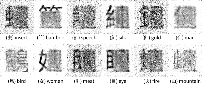
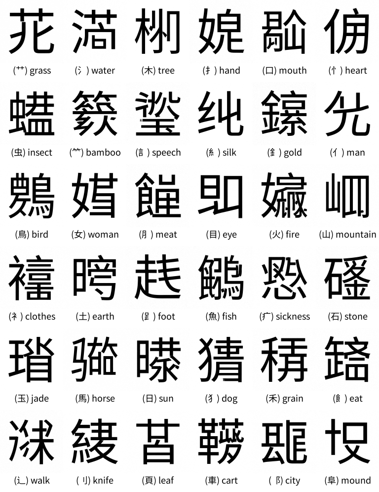
If we obtain a list of most common Chinese radicals from, say, an 18th century Chinese dictionary we can probe the model with prompts corresponding to the English meaning of each radical and see what is activated. Below we take the first sampling step (NB: in the animation in the previous section, we show training steps but each frame is sampled for 50 steps. Don’t get these confused!) for English text prompts corresponding to the most frequently appearing 36 Chinese radicals. (The radicals are not used in the prompt but shown in parentheses for reference):

Very interesting! We see in most cases the corresponding radical is directly activated in the part of the character it usually resides, even though the rest of the character is very noisy. We can infer that the english prompt is strongly tied semantically, i.e. in meaning, to characters that contain this radical.

The 虫 radical means “bug” and is quite strongly activated by the prompt ‘insect’ as it is used in bug-related characters (fly: 蝇, butterfly: 蝴蝶, earthworm: 蚯蚓). However, the 忄(heart) radical is not activated by “heart” (its literal meaning) as its semantic meaning is linked to the historical belief that thoughts and emotions arise from the physical heart (memory: 忆, afraid: 怕, fast: 快). Can we activate this radical by changing our prompt?

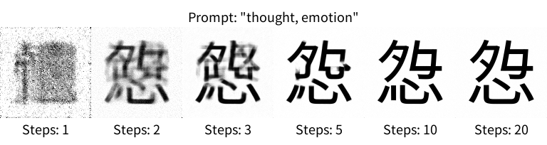
The picture shows sequential sampling (i.e. denoising) steps on the same prompt. While at step 1 we see the model faking toward 忄, it rapidly switches to having a 心 at the bottom. If you can read Chinese, you’ll already know why this is: 忄 is actually an alternative form of 心, which is standalone character for heart and can also be used as a bottom radical. Characters with this radical are also linked to thoughts and feelings, e.g. 念 (to miss) and 想 (to think).

Notably, we can’t access the phonetic component in this model as we haven’t included any information on Chinese pronunciation in the training process. Can we, however, generate new characters using semantic components? Let’s try:

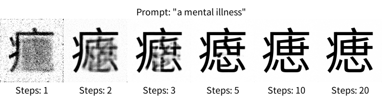
We can! We have both the components for ‘sickness’ and ’thoughts/feelings’ in this character. The overall structure of this character likely draws from characters such as 痣 (zhì, a mole/mark on the skin) in the training set, but in 痣 the 志, also pronounced zhì, is a phonetic component and has no semantic significance. Of course, this is a cherry-picked example. What happens if we try to activate two radicals that prefer to live in the same place? If we provoke a conflict by prompting “a sickness of fire”, for example, we get this:

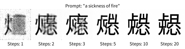
You can see that the model initially tries to place 火 on the left side of the square. By step 3, we can see the sickness radical 疒 also trying to form. As the sampling converges, however, neither concept is strong enough to dominate so the model resorts to enforcing some local structure out of the noise, with the overall character looking not at all convincing.

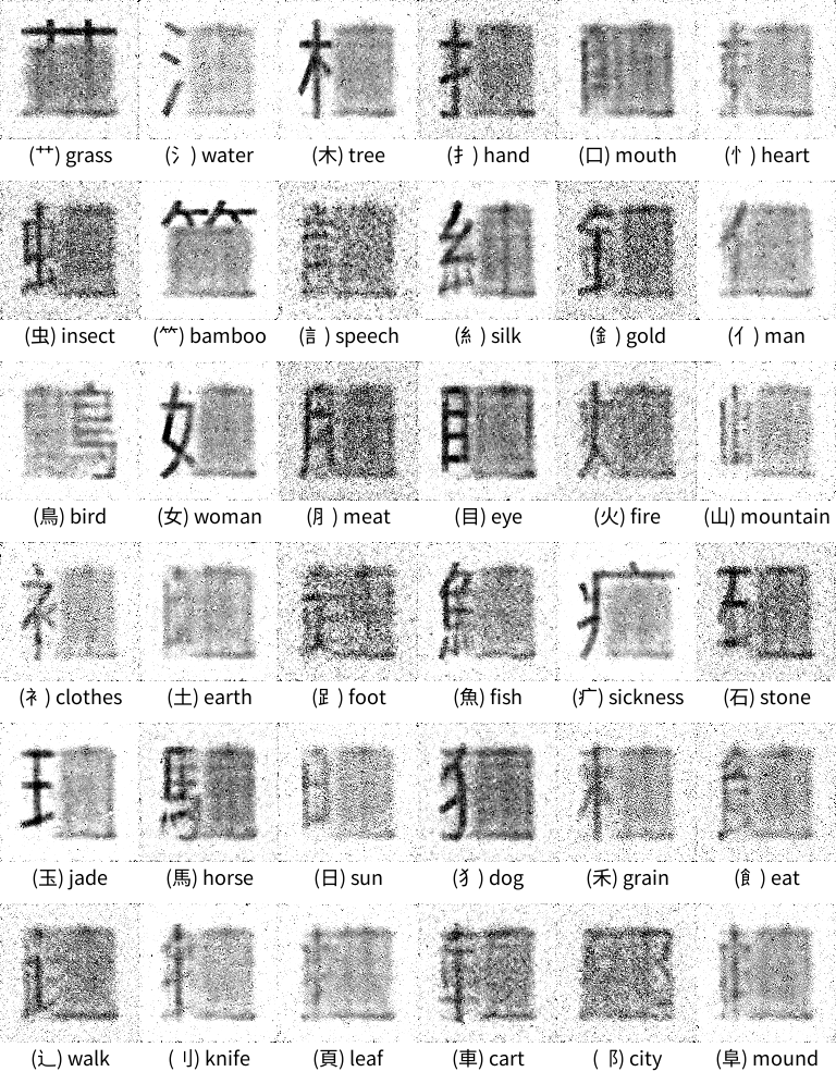
Now that we understand better how the model works, let’s take another look at previous grid and take it all the way up to 50 sampling steps. You may wonder why we never generate the base character, always the radical. The nature of our training set means that there are many more semantically-related training samples containing the radical compared to the one original character, so it makes sense that model would prefer to place the radical in the appropriate position. Sample weighting by corpus frequency would be one way of getting around this! We also see the the rest of the character is filled with what appears to be random stuff. I suspect this is again the model enforcing local consistency without particularly strong semantic guidance.

I tested an implementation including phonetic radical embeddings but there are some structural reason it did not work well - I discuss this here.

Classifier-free guidance (CFG) for the glyffuser

Classifier-free guidance is an elegant and powerful technique that is now used in basically all production conditional diffusion models to improve adherence to prompts. (For an excellent treatment, see here)

Essentially, this method allows the strength of any given prompt to be varied without needing to perform any additional training. Moreover, the strength of the prompt can be increased far above that for standard conditional training. Can we use this method get better generations from the glyffuser?

To implement this method, we simply add random dropout of the text conditioning tokens during training (10-20% has been found to work well). This effectively trains an unconditional model at the same time. During sampling steps, we then perform the noise prediction twice, once normally and once with a blank conditioning tensor. We then combine them as follows:

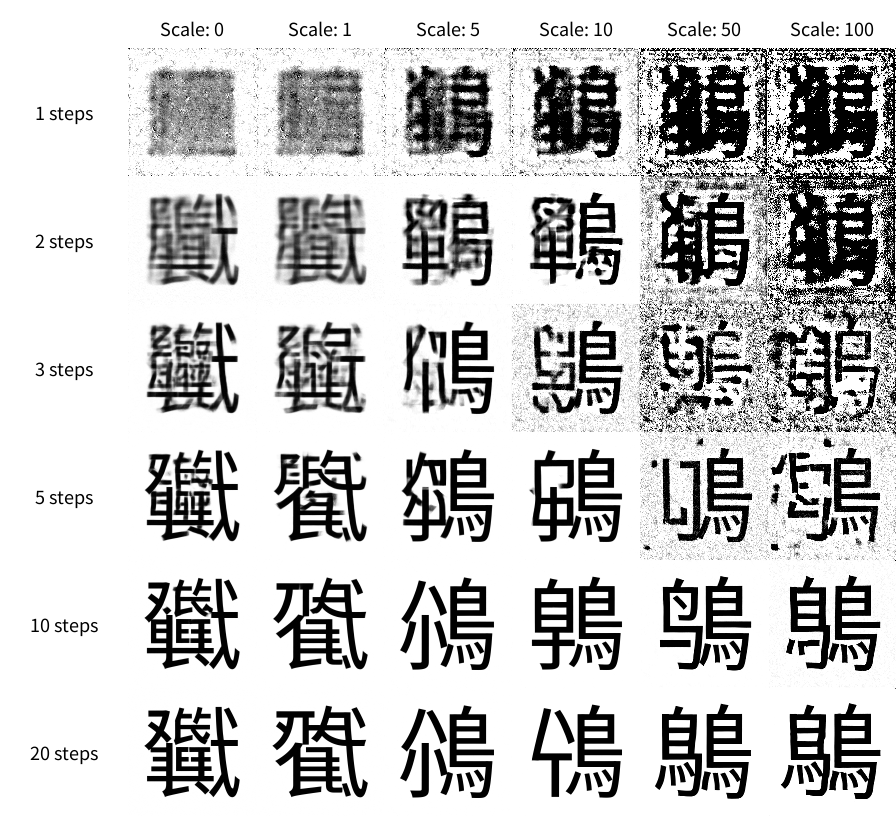
noise_prediction = noise_prediction_unconditional + guidance_scale * (noise_prediction - noise_prediction_unconditional)

Generally, increasing guidance_scale in text-to-image models decreases variety while increasing adherence to the prompt. Let’s try probing the model by varying the number of sampling steps and guidance scale for the prompt “bird” corresponding to a very common radical (鳥/鸟):

I’ve also include interactive explorers for the prompts ‘fire’ and ‘hair’ in the appendices. I highly recommend taking a look, they are very funny!

Compared to the base conditional model, we see that as we increase the guidance scale, the ‘bird’ radical becomes increasingly activated from the very first sampling step. Interestingly, while the traditional form of the bird character “鳥” dominates (it is more prevalent in the training set), the simplified form “鸟” also makes a single appearance (10 steps, scale=50), making it a ’transition state’ during the denoising process. The explorer below shows CFG scales of 0 to 100 for different random seeds - higher CFG scales do indeed reduce sample variety. Compared to general-purpose text-to-image models however, we can tolerate higher CFG scales as they tend to give more convincing characters. If you follow any individual character, you’ll see that it tends to start with one ‘bird’ radical, then as CFG scale increases, at some point the other side will also collapse to a ‘bird’ radical.

Looking at the a picture of varying CFG scale generations for prompts for each common radical below, we see that for scale values of around 5-15, the generated characters are much more consistently convincing than the those made by the base conditional or unconditional models. (I think that anyone who grew up with Chinese or has studied it for a long time gains a strong instinctive sense of whether a character could be real, even if they don’t recognise it.)

Outro

So can we teach a model to understand how Chinese characters and then invent new ones? It looks the answer is a resounding yes! We find that the final conditioned diffusion model (the Glyffuser™) has a strong conception of how the components of a Chinese character relate to its meaning, in much the same way a human would guess at the meaning of an unknown character. Moreover, by strengthening the adherence to known concepts using classifier-free guidance, we can generate very convincing characters that follow the rules of Chinese glyph construction.

Test the models here

If you want to try out the conditional glyffuser, the easiest way is to get the demo repo with git clone https://github.com/yue-here/glyffuser, make a python environment with requirements.txt (you may need to set it up for your GPU and jupyter) then run the glyffuser inference.ipynb notebook, which will summon the trained model from my huggingface repo.

Failing that, I’ve made this applet that will run the inference, but please be patient as it’s quite slow (around a minute per step).

Appendices

Appendix 1: other writing styles

Here’s a training video from a version of the glyffuser trained on the ancient Chinese writing known as seal script:

Appendix 2: phonetic radicals

To include the phonetic radicals, we need a representation. The standard romanization is known as pinyin - for example, the phrase 人工智能 (artificial intelligence) would be “rén gōng zhì néng”. The diacritics on the vowels are the tones of which there are 4 in standard mandarin. These can also be represented numerically, e.g. “ren2 gong1 zhi4 neng2”.

Simply adding the pinyin to the english definition prior to training is unlikely to work as we are using a frozen tokenizer and text model which does not recognize the pinyin syllables. Instead, we can create separate embeddings of the same length as the image vector for the pinyin and add them directly, the same as the text conditioning is added. Specifically, based on how Chinese syllables are structured, I added 3 trainable embeddings for the initial, final, and tone (for example, ren2 would become ‘r’, ’en’ and ‘2’). To train the model, I added extra inputs for the pinyin and tone.

After training the model in the same way as before, I tried to ‘summon’ the phonetic components. However, the results only changed slightly with different pinyin prompts. I suspect this is because of the excessive homophony in Chinese. For example, 羊 (yang2, ‘goat/sheep’) is a common phonetic radical. But for this exact syllable, wiktionary gives 47 different characters. Have a look at characters containing the top two phonetic radicals for this pronunciation, 羊 and 昜:

羊佯垟徉样洋烊珜眻蛘𨦡羏劷
昜崵揚暘楊湯敭瑒煬禓瘍諹輰鍚鐊陽霷颺鰑鸉

It’s likely the same situation as the ‘clashing radicals’ case where we can’t activate the ‘fire’ and ‘sickness’ radicals at same time - when neither phonetic radical dominates the distribution, we end up sampling garbage.

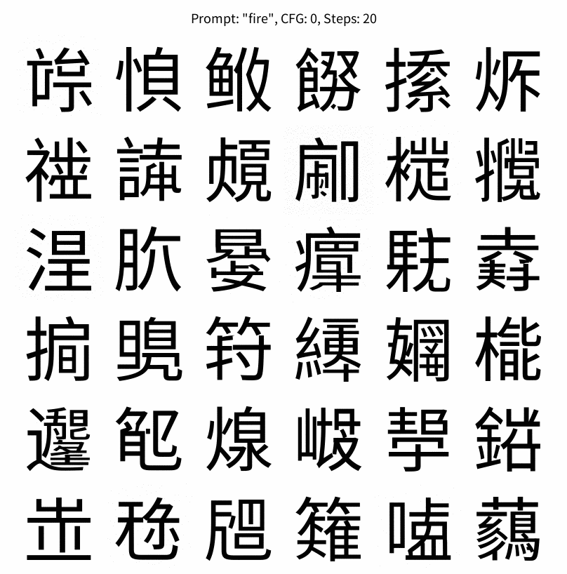
Appendix 3: CFG variations for “fire”

The Chinese character for fire “火” has a particularly varied set of possible locations. These are showcased in the characters “炎” and “焱”. Another form is the bottom radical “灬”, a kind of deconstructed version of “火”. As such, greater variety is possible and this shows:

Appendix 4: CFG variations for “hair”

I’m mostly including this because the characters look very funny.