Optical flow timelapse stabiliser
Using computer vision to stabilise timelapse footage
For associated code, please see the Jupyter notebook in the github repository
While machine learning has been very successful in image-processing applications, there’s still a place for traditional computer vision techniques. One of my hobbies is making timelapse videos by taking photos every 10 minutes for many days, weeks or even months. Over this time scale, environmental effects such as thermal expansion from the day-night cycle can introduce period offsets into the footage. I have a backlog of timelapse footage that is unwatchable due to excessive shifts of this nature. In the past I’ve used the Blender VFX stabilization tool to stabilize on a feature, but this breaks in e.g. day-night cycles or subjects moving in front of the feature. I finally got round to writing my code to do this that doesn’t rely on specific feature tracking.

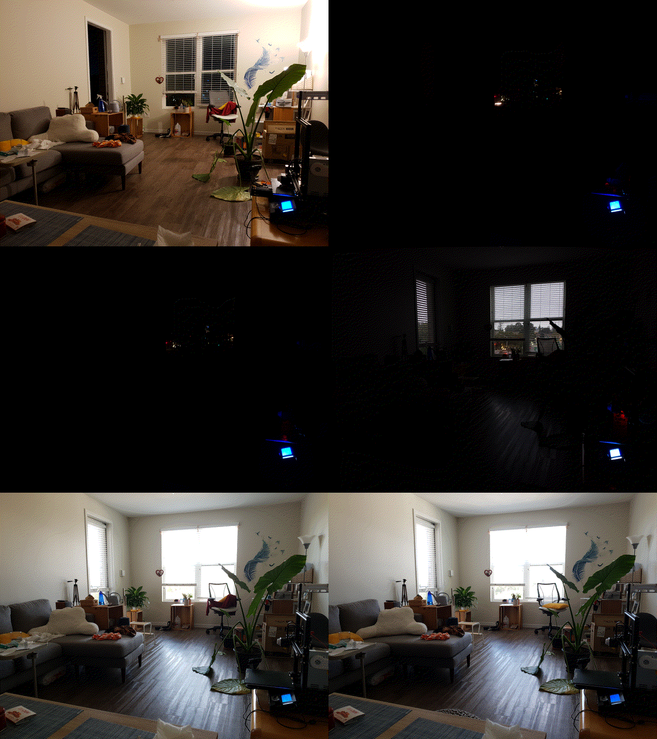
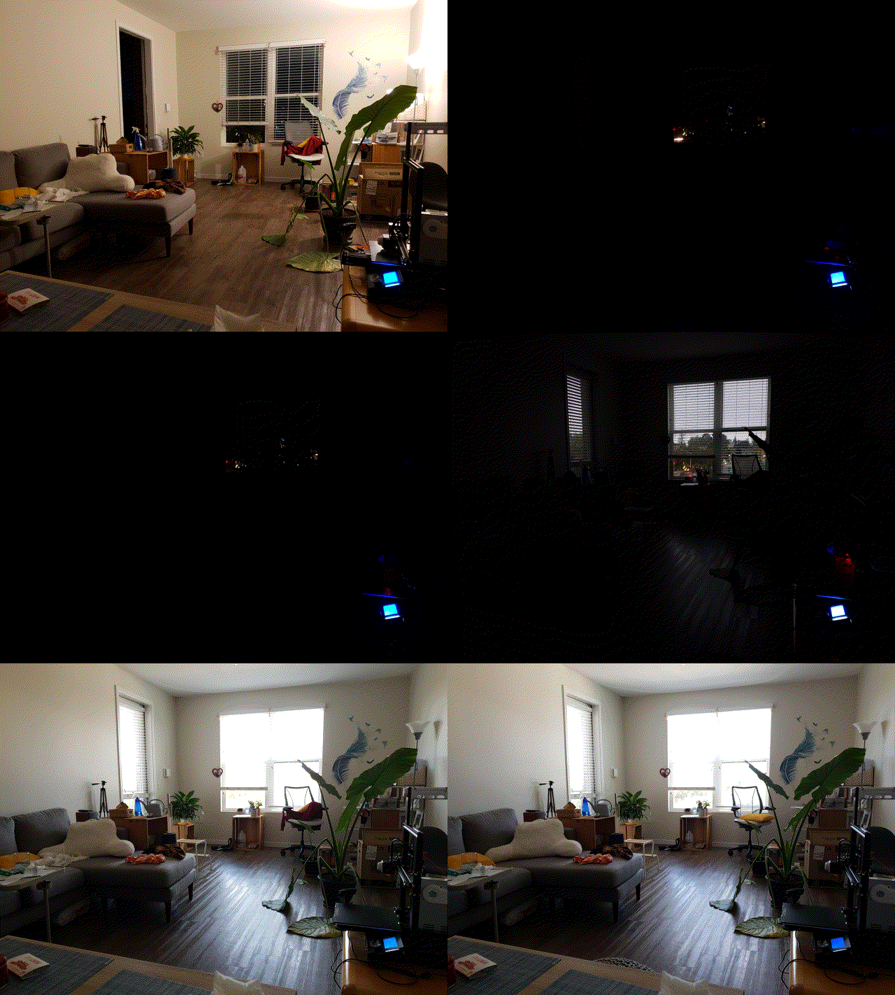
A short clip of unstabilized footage
Background
I had a vague conception that tracking a similarity metric between two frames would furnish the shift between then, perhaps using least-squares peak fitting in a similar way to the fitting of X-ray diffraction data (once you have a hammer, everything looks like a nail!) by performing gradient descent with small shifts to the two frames.
To my great relief I didn’t have to write this code as further investigation revealed OpenCV contains a feature called optical flow which essentially performs this calculation, outputting vectors for the movement of every pixel between two frames. This could form the basis of stabilisation code.
Execution: optical flow interpretation
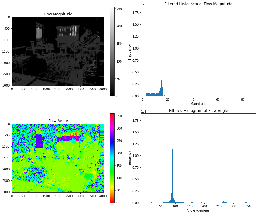
My exploratory calculations showed that the optical flow vectors did indeed provide a clear picture of shift direction and magnitude.

Optical flow analysis of a frame transition with a small shift downward
You can see in the maps above the algorithm detects pixels that can be mapped to a clear shift (furniture etc.) while uniform areas like wallpaper aren’t picked up. The regions of uniform grey in the “flow magnitude” plot indicate a consistent shift, and the sharp peak in the histogram of shifts confirms this - the camera view has tilted by around 16 pixels. Likewise for the “flow angle plot”, the peak in the histogram at ~90° indicates a shift downwards.
The next step was to work out how to use these results. It was clear that this was already a relatively expensive calculation and it would have to be performed on ~18,000 pairs of frames for my test timelapse dataset.
(Aside: luckily, OpenCV has easily accessible GPU acceleration with OpenCL. Simply replacing standard matrices with UMat objects speeds up the calculations by an order of magnitude. I looked into using the CUDA implementation which would likely be even faster, but it seemed more trouble than it was worth to install.)
While peak fitting the histograms would yield the best result in principle, I opted for an economical approach to save compute: filter out magnitudes that were the first entry in the array (i.e. the top of the decay curve, not a peak), only include angles within 5 of 90/270 degrees (i.e. vertical shifts), then take the max values and round the angles to 90 or 270.
This part was done as a single script outputting a CSV file of the 4 relevant parameters extracted from histograms for each frame - vector magnitude, vector angle, and the frequencies of each . (In principle the full optical flow vector set could be saved but file would be huge. The 17K frame dataset took around 90 min on my system which was an acceptable tradeoff for repeats.)
Execution: stabilisation
This part was simple in principle but somewhat difficult in practice. The idea was very simple - by cropping the top and bottom of each frame by the maximum total shift across the dataset, the relative shift of each frame could be controlled by varying the shifts above and below.
The execution: Calculate the relative shift from the starting position at for each frame of the dataset by summing the up and down shifts. The overall window size across the set can be extrapolated by the distance between the maximum and minimum shift. Then for the starting frames, crop down to the window size. Afterwards, perform the first crop plus the relative shift calculated previously to shift the visible window to a consistent location. It’s difficult to explain clearly but the code and demonstration make it clearer.

